seasonal 1.10: R-interface to X-13ARIMA-SEATS

time-series

Author

Christoph Sax

Published

October 21, 2024

We are happy to announce that the latest CRAN version of seasonal fixes several bugs and makes it easier to read specialized output from X-13ARIMA-SEATS. See here for a complete list of changes. In addition, the accompanying seasonalview package has been updated and finally gets rid of some annoying warning messages.

What is seasonal adjustment?

Time series data often display recurring seasonal patterns throughout the year. For instance, unemployment rates in the United States typically rise from January to March and again in June and July. By applying seasonal adjustment, analysts can identify and remove these predictable annual patterns, allowing for clearer interpretation of fundamental changes in the data. The R package seasonal provides a powerful and user-friendly way to perform this task in R, leveraging the X-13ARIMA-SEATS procedure developed by the U.S. Census Bureau.

Getting started in R

To get started, use the seas function on any time series:

library(seasonal)
m <- seas(AirPassengers)
summary(m)


Call:
seas(x = AirPassengers)

Coefficients:
                    Estimate Std. Error z value Pr(>|z|)    
Weekday           -0.0029497  0.0005232  -5.638 1.72e-08 ***
Easter[1]          0.0177674  0.0071580   2.482   0.0131 *  
AO1951.May         0.1001558  0.0204387   4.900 9.57e-07 ***
MA-Nonseasonal-01  0.1156204  0.0858588   1.347   0.1781    
MA-Seasonal-12     0.4973600  0.0774677   6.420 1.36e-10 ***
---
Signif. codes:  0 '***' 0.001 '**' 0.01 '*' 0.05 '.' 0.1 ' ' 1

SEATS adj.  ARIMA: (0 1 1)(0 1 1)  Obs.: 144  Transform: log
AICc: 947.3, BIC: 963.9  QS (no seasonality in final):    0  
Box-Ljung (no autocorr.): 26.65   Shapiro (normality): 0.9908

By default, seas calls the automatic procedures of X-13ARIMA-SEATS to perform a seasonal adjustment that works well in most circumstances.

To extract the final series, use the final() function:

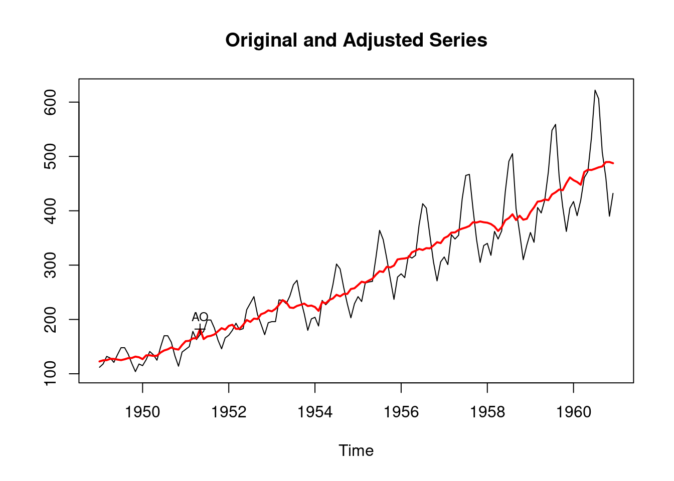
final(m)

To plot the results, use the plot() function:

plot(m)

Input and output

In seasonal, it is possible to use the complete syntax of X-13ARIMA-SEATS. The X-13ARIMA-SEATS syntax uses specs and arguments, with each spec optionally containing some arguments. For example, in order to set the ‘variables’ argument of the ‘regression’ spec equal to td and ao1999.jan, the input to seas can be specified like this:

m <- seas(AirPassengers, regression.variables = c("td", "ao1955.jan"))

seasonal has a flexible mechanism to read data from X-13ARIMA-SEATS. With the series function, it is possible to extract any output that can be generated by X-13ARIMA-SEATS. For example, the following command returns the forecasts of the ARIMA model as a time series:

m <- seas(AirPassengers)
series(m, "forecast.forecasts")

Graphical user interface

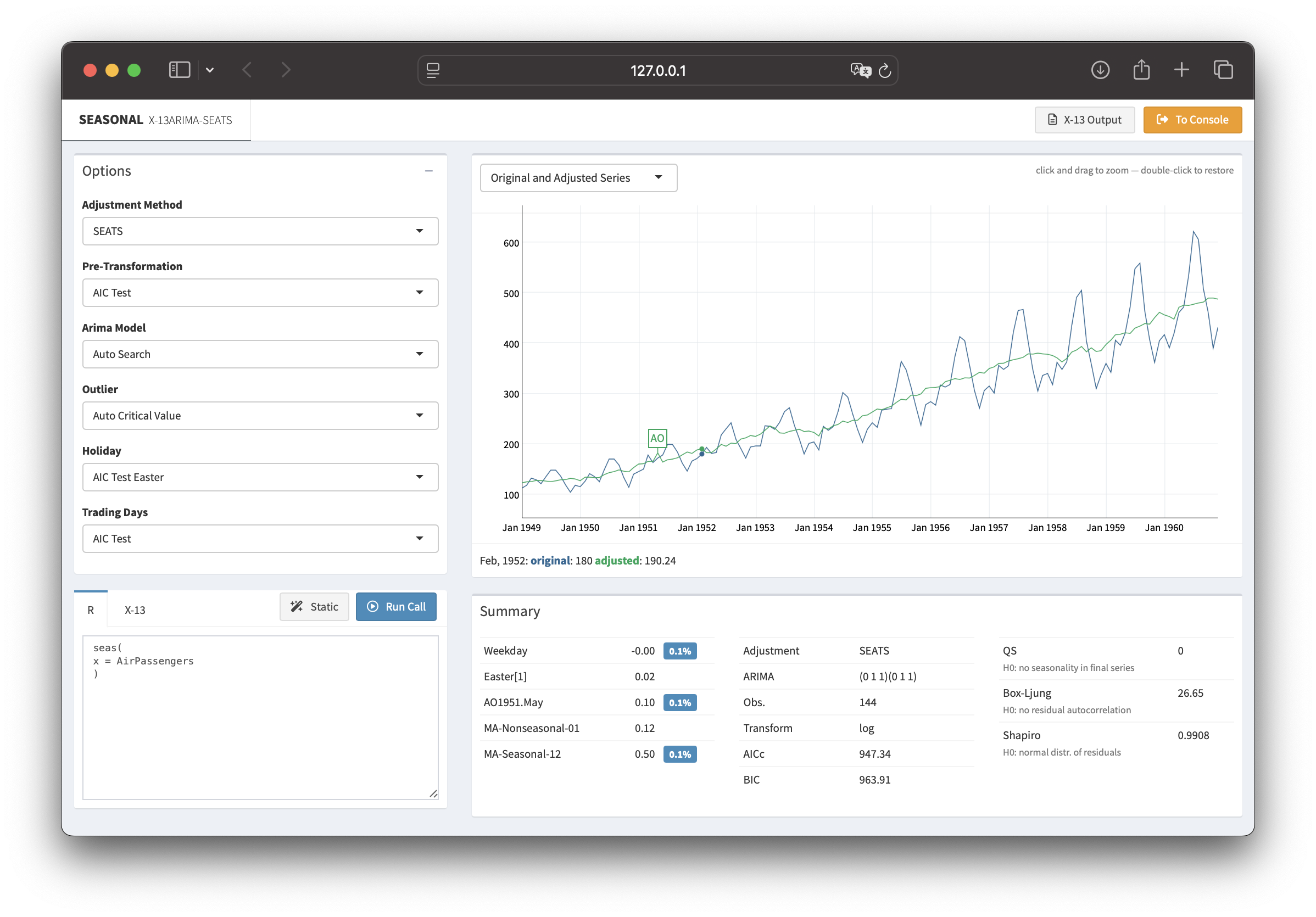
The seasonalview package provides a graphical user interface to explore the results of the seasonal adjustment. Use the view() function to open it:

view(m)

This interface allows for interactive exploration and adjustment of seasonal models, making it easier to fine-tune your seasonal adjustments and visualize the results.

More information

For a more detailed introduction, check our article in the Journal of Statistical Software or visit the package website. The package website also allows you to upload your own data and explore the results interactively.

You can report bugs, ask questions, or contribute to the development on our GitHub repository. Thanks for using seasonal!